In this notebook, we compute taxes, rates and marginal rates of the German tax system. The computations are based on the official rates in 2010-2014 (no responsibility for the correctness).
>function  map tax (x:scalar, married:integer=0) ...
 if married then xs=x/2; f=2; else xs=x; f=1; endif
 if xs<8130 then return 0
 elseif xs<13470 then y=(xs-8130)/10000; return (933.7*y+1400)*y*f
 elseif xs<52881 then y=(xs-13470)/10000; return ((228.74*y+2397)*y+1014)*f
 elseif xs<=250730 then return (0.42*xs-8196)*f
 else return (0.45*xs-15718)*f
 endif
 endfunction
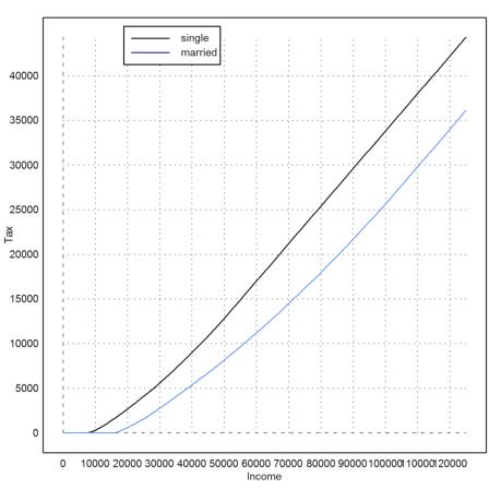
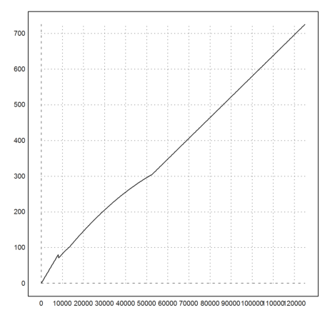
The following plot shows the increase of the tax with the income.
The convexity of the function is called progression. The result is that the marginal rate is slowly increasing too.
In germany, married couples share their income. The income is divided by two and the tax is twice the tax for half of the income. Thus the lower blue curve is the tax rate for married couples with the combined income.
>plot2d("tax",0,125000); plot2d("tax";1,add=1, color=12); ...
 xlabel("Income"); ylabel("Tax"); ...
 labelbox(["single","married"],colors=[black,blue],x=0.4):
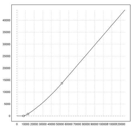
In the following plot, we mark the seams between the parts of the tax function.
>plot2d("tax",0,125000); ...
 x=[7664,12739,52151,250000]; y=tax(x); ...
 plot2d(x,y,points=true,add=true):
The rate of the tax is the proportion of the income you have to pay for taxes.
>function taxrate (x,married=0) := tax(x,married)/x
Example.
>print(taxrate(30000,1)*100,2,unit=" %")
9.24 %
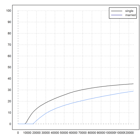
The following plot compares the tax rate of single and married income.
>plot2d("taxrate(x)*100",a=1,b=125000,c=0,d=100); ...
 plot2d("taxrate(x,1)*100";1,add=1,color=12); ...
 labelbox(["single","married"],colors=[black,blue]):
The marginal tax rage is the derivative of the tax rate. It is the rate, at which additional income is taxed.
An example: A married couple get 1000 Euro more starting from 30000 Euro. Then about 25% of this goes to tax.
>(tax(31000,1)-tax(30000,1))/1000->" %"
24.7843144 %
We compute the marginal tax rate simply by numerical differentiation.
>function marginaltaxrate (x,married=0) := diff("tax",x;married);
>marginaltaxrate(30000,1)->" %"
24.6699442118 %
Let us add the marginal tax rate to our plot.
>plot2d("marginaltaxrate(x)*100",add=1,style="--"); ...
 plot2d("marginaltaxrate(x,1)*100",add=1,color=12,style="--"); ...
 labelbox(["rate","married","marginal","married"], ...
   colors=[black,blue,black,blue],styles=["--","--","-","-"]); ...
 xlabel("I"); ylabel("%"):
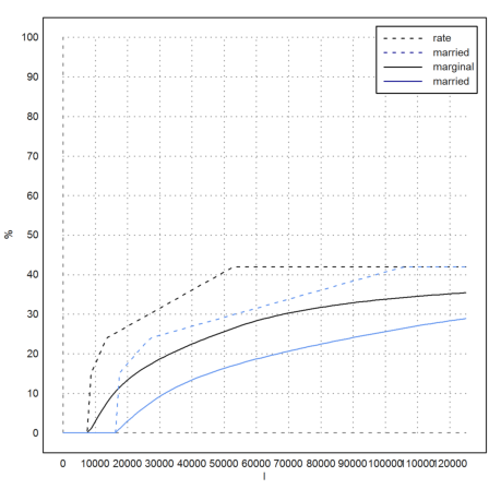
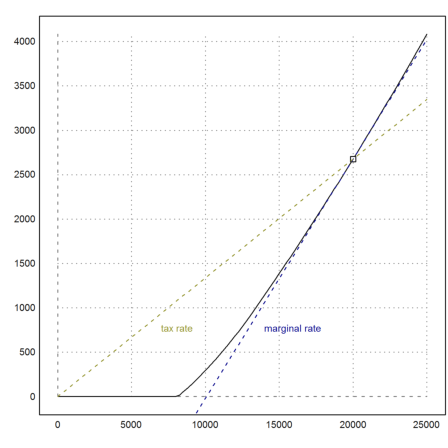
The marginal tax rate is the slope of tangent, the tax rate the slope of the lien through (0,0).
>plot2d("tax",0,25000); ...
   x0=20000;  plot2d(x0,tax(x0),points=1,add=true); ...
   plot2d("tax(x0)+marginaltaxrate(x0)*(x-x0)",color=4,add=true,style="--"); ...
   plot2d("tax(x0)+taxrate(x0)*(x-x0)",color=6,add=true,style="--"); ...
   label("marginal rate",13500,900,color=4); ...
   label("tax rate",6500,900,color=6):
The elasticity of the tax tells us the increase of the tax in percent versus the increase of the income in percent.
>function taxelasticity (x,mar=0) := marginaltaxrate(x,mar)*x/tax(x,mar); ...
 plot2d("taxelasticity",10001,125000):
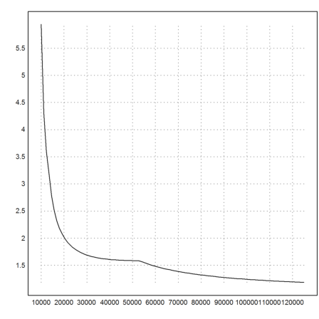
This plot shows that higher incomes seem to profit more from percentage raises in terms of relative tax increase. But the actual increase of the net income is more important.
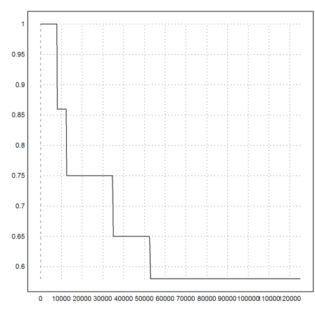
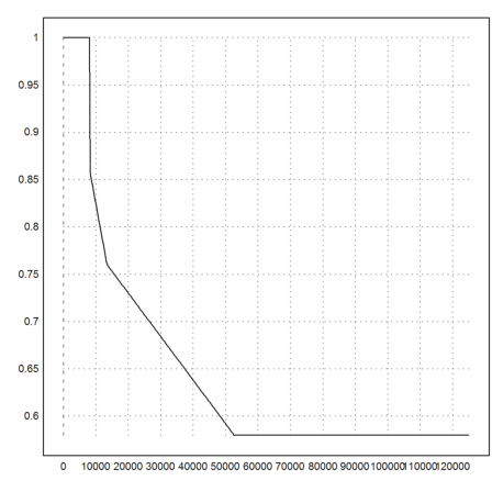
So let us compute the percentage of the gain after taxes for a 1% raise before taxes. As an example, very low incomes will gain the total of 1%, since they do not pay taxes.
>plot2d("(x*0.01-(tax(x*1.01)-tax(x)))/x*100",1,125000,n=500):
In absolute numbers, we can compute the gain after taxes for a 1% raise before taxes.
>plot2d("x*0.01-(tax(x*1.01)-tax(x))",1,125000,n=500):
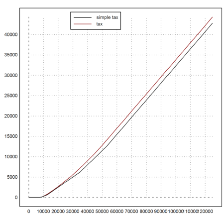
For comparison, we compute a more simple tax system, which has been proposed recently.
The difference to the existing system are constant marginal rates. We take rates of 14%, 25%, 35%, 42%, 45% for incomes over 8000, 12500, 35000, 53000, 250000 Euro respectively.
>function map S(X) ...
 S=0;
 if X>=250000 then S=0.45*(X-250000); X=250000; endif;
 if X>=53000 then S=S+0.42*(X-53000); X=53000; endif;
 if X>=35000 then S=S+0.35*(X-35000); X=35000; endif;
 if X>=12500 then S=S+0.25*(X-12500); X=12500; endif;
 if X>=8000 then S=S+0.14*(X-8000); endif;
 return S;
 endfunction
Here is a comparison of the simple and the official tax.
>plot2d("tax",1,125000,color=red); plot2d("S",>add);  ...
   labelbox(["simple tax","tax"],colors=[black,red],x=0.5):
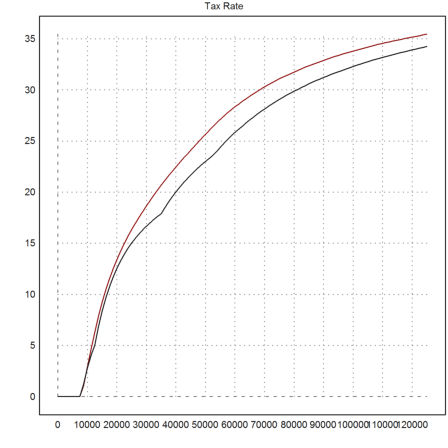
The tax rate is still increasing.
>function SS(X) := S(X)/X; ...
 plot2d("taxrate(x)*100",1,125000,color=red,title="Tax Rate"); ...
 plot2d("SS(x)*100",add=1):
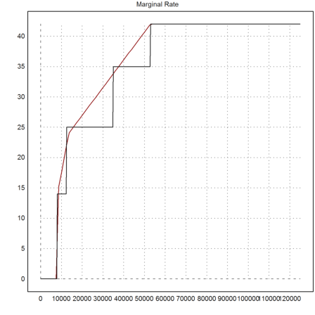
The marginal tax rate is discontinuous now, compared to the old continuous marginal rate.
>function dS(X) := diff("S",X); ...
 plot2d("marginaltaxrate(x)*100",1,125000,color=2); ...
 plot2d("dS(x)*100",add=1,n=500,title="Marginal Rate"):
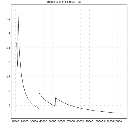
The elasticity looks weird now.
>function SE(X) := dS(X)*X/S(X); ...
 plot2d("SE",11000,125000,n=500,title="Elasticity of the Simple Tax"):
What is left of a 1% raise before taxes?
>plot2d("(x*0.01-(S(x*1.01)-S(x)))/x*100",1,125000,n=500):